
I spent 1 year trying to predict company growth from SEC filings. It failed.
Going super deep into the financial NLP rabbit hole.

What about feeding whatever unstructured data you have about a company (full text of SEC filings or company website) into a custom encoder transformer, and have it output a quantitative prediction of its 5y growth rate?
That was my ultimate goal.
To get there, I had to teach a transformer how to understand numbers, train it to encode entire documents into a single embedding (and only keep what’s most interesting about said document), and use the embedding to try to predict the growth rate.
The prediction part failed. The rest is a success, and it can be used elsewhere.
Why unstructured data should carry signal
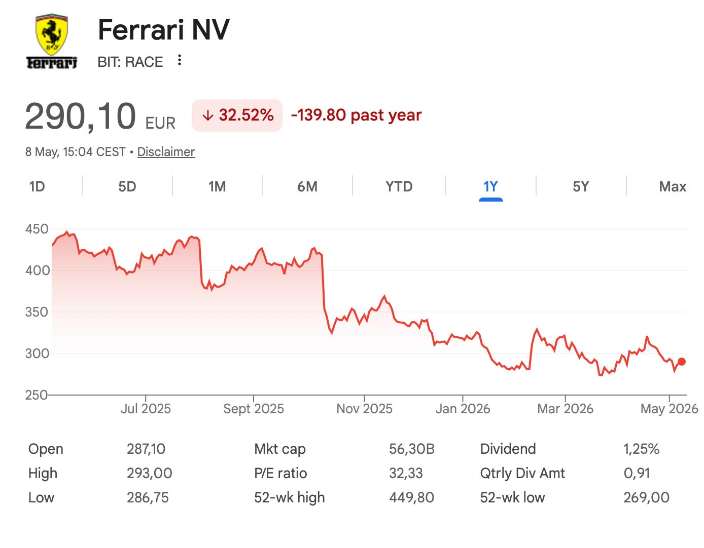
When I first checked Ferrari’s website, I was astonished. I had never seen a website so bad. I believe it would have been better for them to put a warning page reading “Dear customers, if you like cars, get lost. We, the top management and marketing team, decided that you’d rather watch strobing 480p videos of people carrying handbags with the Ferrari logo on them”.
There’s no way such a website is compatible with a healthy top management. A sane CEO would have set the marketing department on fire, sent an apology letter to every would-be customer, and gone on a pilgrimage to reflect on his sins.
I think the website of a company is the best public window to its inner workings. Like the way someone looks and speaks can tell you a lot about their psychology.
Also, I believe that the text of financial data gives a lot of information. If you see a footnote reading “we used mark-to-market accounting for our long term, nonfinancial contracts (but don’t worry, everything’s gonna be alright)”, you’d better be careful.
When it comes to financial analysis, there’s a no man’s land between what statistical models can do, and what humans can do. The former have been trained on 100,000s of datapoints but have a very shallow understanding of finance. The latter have been trained at most on 1,000s of datapoints (financial statements and business stories), but have a deep understanding of how things work.
LLMs have started bridging that gap, starting from the human side. Claude can help you analyze a financial statement, and would flag obviously fishy footnotes. But it hasn’t been trained to say “On average, companies with such an income statement grow 1.53% in the next year”.
This project is about trying to bridge the gap starting from the other side: a statistical model that’s more intelligent than a random forest, yet still trained on a lot of datapoints.
Thing is, there are a lot of technical hurdles to get there. First one is that text transformers are bad with numbers.
Ask an LLM: how close is 9,234 to 9,235?
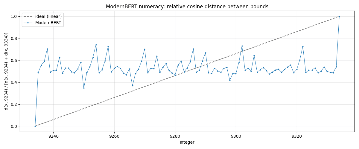
I wouldn’t bet my ass on a financial model that has no clue how to sort numbers.
The problem is that ModernBERT’s1 tokenizer treats numbers as discrete tokens, and breaks them down nonsensically. For example, 1000 gets tokenized as ‘100’, ‘0’, whereas 999 gets tokenized as ‘999’. How is the model supposed to figure out that these 2 numbers are close together, despite sharing 0 common tokens?
The training objective (predicting masked tokens with CE loss) is not really suited for this task either. It rewards exact prediction, not a “hmmmm, the number I have to predict should be around 1,000”. Sure, with enough parameters and enough training tokens, one could get a decently performing transformer. But the inductive bias of the default architecture is just not suited for the job.
There are a few existing methods to tackle these problems, but I don’t like them2.
Step 1. Making ModernBERT good at numbers
< deep dive>
After a few weeks of experimentation, here’s the best strategy/architecture I came up with:
Encoding numbers in log-magnitude. Most of the time, in financial data, the relative uncertainty is more important than the absolute one. No one cares if Apple’s revenue is $416.161B or $416.162B, but everyone cares if their EBITDA margin is 0% or 1,000,000,000% (same absolute uncertainty). I chose to encode numbers from 1e-3 to 1e123, a 16 OOM window.
Breaking up the 16 OOM window into 128 bins, with linear interpolation.
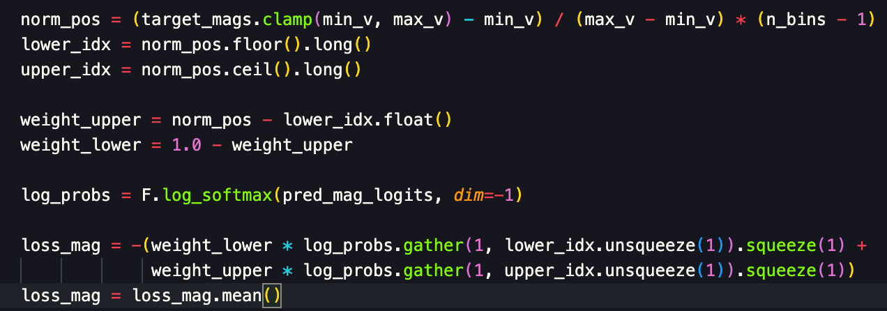
Encoding (embedder): An embedding dict maps each of these 128 bins to a learned 768-dim (ModernBERT’s hidden dim) vector. It’s basically a free (flop-wise) set of parameters. As nearly all numbers fall between 2 bins, a linear interpolation of the 2 closest bins is performed4.
Decoding (prediction head): Classification-regression using the same 128 bins, with linear interpolation too. A simple MLP(last_hidden_states) with an output dim of 128 did okay, but I decided (maybe not the best call5) to use a GLU approach that performed a bit better. Smooth Cross-Entropy loss on the 2 closest bins6.
</deep dive>
I iterated quickly on this architecture by full-fine-tuning ModernBERT on a synthetic numeracy dataset, that tested the model’s ability to perform simple arithmetic operations on 1e-4 to 1e6 numbers, in natural language. Like “16 plus 24 gives [MASK]”, or “If you divide 1,234,345 by 567, you get [MASK]”, or “45 minus [MASK] gives 34”. I believe I spent around $30 of compute on these experiments.
The best architecture was able to predict the results with an MRE of around 10% after 30 L4-minutes on this toy dataset.
Then, I tested it on a real (though heavily formatted) dataset, that I synthesized from structured financial data that I got for another one of my projects. Results were impressive (MRE was about 5% or so, despite some numbers being quite difficult to infer from others).
So, at that point, I had a backbone model I knew would be good at numbers. But I had no data yet.
Step 1.2 Data acquisition and sanitization
Although this part is the most important of the whole blog post, it’s not the most conceptually interesting (despite a few tricks that I’m quite proud of). So, I discuss it in the annex. You can check it there if you want.
The final dataset is composed of:
All 2018 10-K filings
All AA accounts for all 50+ employees British companies (2018)
A wikipedia regularization dataset (100M tokens)
I appended website statistics (not their full texts, as I wanted to first check how the model would perform on statistics, that are arguably more information dense than the full website), to all company filings for which I could find the website archive as of 2018.
Everything was heavily curated and sanitized. You can check the annex for more information.
316M tokens dataset in total. Full dataset available here.
Growth rate was defined as an average of multiple growth figures: Employee count, revenue, net income… You can check the weights of this average here.
I can’t stress enough that good data matters much more than a good architecture. And that spending a few hours on data sanitization yields better results than spending 100s of hours tweaking the number of attention heads of a transformer.
Step 2. Training the backbone model on real data
So, after I obtained and sanitized all the 2018 SEC and companies house filings (>50 employees) and websites, I proceeded with the MLM training (predicting masked tokens in a sequence) of the model on that 300M tokens dataset7. The main objectives were:
Specializing the model on financial data
Teaching it how to handle numbers with its new number embedder/head
I started off using complex LoRA setups with warmup phases where I froze everything but the number-specific part of the model. Classic “I’m gonna over-engineer it” mistake. Full fine-tuning gave much better results. I just used a decent chunk of English Wikipedia for regularization, so that the model doesn’t catastrophically forget all its pre-training.
So, decent improvement above baseline. Training took around 2h on an RTX 6000 Blackwell. You can check a full SEC filing inference example here, just to get a vibe-sense of what these numbers mean. Loss comparison is irrelevant here because of the tokenizer change8.
The (trained) model is published on HuggingFace here. For more information on the training setup and failed experiments, please contact me if needed9.
So, at this point, we have a model that (superficially, it only has 150M params) understands finance, and numbers. But it’s not good at distilling a sequence, let alone a whole document into a nice vector that we can use for quantitative analysis10.

Step 3. Making the backbone into a document embedding model
This is the tricky part.
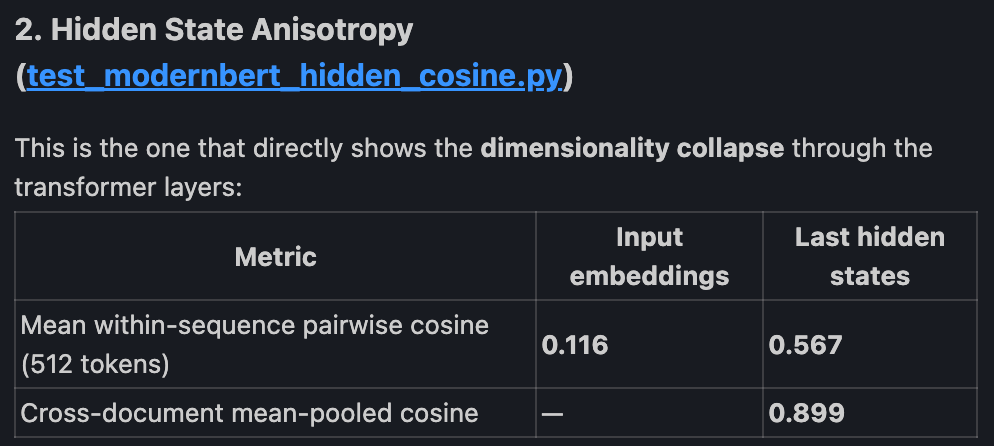
When a model has been trained to predict masked tokens, its last hidden states are quite informative, but they also contain specific details about the tokens to predict, that are irrelevant for sentence embedding purposes. Also, there’s a tendency of transformers to collapse the effective dimensionality of their outputs compared to their inputs11.
So, I really had to fine-tune the backbone model into a sequence embedder, to make it:
Better at encoding relevant sequence information, without all the token-prediction noise.
Better at discriminating between different sequences.
Usually, what you do is that you take pairs of sequences that you want the model to consider “close” (positives), and pairs that are dissimilar (negatives). Like “the company reported strong earning growth in the last quarter” and “our business grew strongly in the last quarter” for positives.
You take their CLS12 embeddings, as well as that of a lot of negative examples, and you do some contrastive learning13.
Thing is, for this to work, you need a lot of positive pairs to train the model upon.
And creating positive pairs is something that comes with a certain bias: you have to decide what, in a sequence, is sufficiently irrelevant to be paraphrased14. I didn’t want to bake such assumptions into the model, so I went for an unsupervised method for making it learn sequence representations. 2 methods, in fact.
3.1. JEPA. It failed. But it’s mathematically elegant.
The core idea of JEPA is quite close to contrastive learning. It’s basically “let’s give the model slightly augmented versions of the same text/image (different crops, different token masks, different dropout masks…) and ask it to output similar embeddings for them. In order to prevent it from collapsing into predicting a constant (which obviously satisfies the previous objective), let’s make the output’s distribution gaussian”15. I like it. I believe it’s the cleanest unsupervised way to make an output distribution both informative and locally consistent.
My “positives” were both augmented versions of the same chunk and different chunks from a given document.
It trained very well: the MSE loss term was really small and the SIGReg term was acceptable16. End model’s embeddings participation ratio was decent (at least 128), everything looked fine.
Problem is that it just didn’t work on my custom STS and ordering benchmarks.
<deep_dive>
I can’t give a definitive explanation for that, except for the obvious “ensuring the model gives consistent representation for very close pairs wasn’t sufficient to make it consistent on less close pairs”17. I believe the problem comes from the fact that different crops from a given image (which JEPA was designed for) are more closely related than different chunks from a given document. And, in my setup, the no man’s land between “incredibly close pairs (augmented versions of the same chunk)” and “vaguely related pairs (different chunks from the same document)” prevented the model from learning a continuous representation of its input space.
</deep_dive>
3.2. Autoencoder setup. Worked fine. But beware of its frequency bias.
Another idea I’ve had after checking the EmbeddingGemma paper was to use the CLS token as a bottleneck carrying information from a sequence encoder (that we want to train) to a decoder (that we don’t care too much about).
Training setup was: giving an unmasked chunk to the encoder, give its CLS representation to the decoder, along with a heavily masked18 version to the chunk, and have it reconstruct the chunk.
Unlike the original transformer paper, I decided to go for a bidirectional decoder, for a few reasons19. Also, unlike that paper, only 1 token (the CLS) was attended to in the cross-attention layers. Which was obviously wrong, and needed to be addressed: softmax(only_one_attention_score) = 1.
So, I asked Claude to come up with an idea, although I had a few of my own. It chose brute force: expanding the CLS token embedding into 16 slots via a different full rank (768*16, 768) transformation for each layer. At first, I thought it was dumb: it more than doubled the param count of the decoder relative to its encoder base model. Plus, 16 full rank projections of a single embedding is as close as it can get to a complete a priori red flag.
But it’s the best decoder I’ve tried20. The condition numbers of each slot transformations are incredibly small21, hinting that it’s a good solution.
The frequency bias of this autoencoder setup, and how to mitigate it <deep_dive>
I liked the fact that this autoencoder setup makes the encoder only care about what can’t be inferred from the context. Seeing a few words from a CYA section is enough to guess all of it. So, the encoder doesn’t need to tell anything about it to the decoder.
But there’s a subtle trap in there. The presence of such boilerplate is in itself an information, and it needs to be preserved. If we take an image analogy, the decoder tries to denoise images, and the encoder thus only has to give high-frequency information to the decoder. Not “this is a landscape picture, and the sky is blue”. This, the decoder doesn’t need to know to denoise a patch from the pixels (tokens) it sees. The decoder doesn’t need it, therefore the encoder isn’t going to encode it. But we still might need it. So, I had to find a way for the low-frequency information (“this picture is a landscape” or “this 10-k comes from an energy trading company with strange accounting practices”) to make its way into the CLS embeddings.
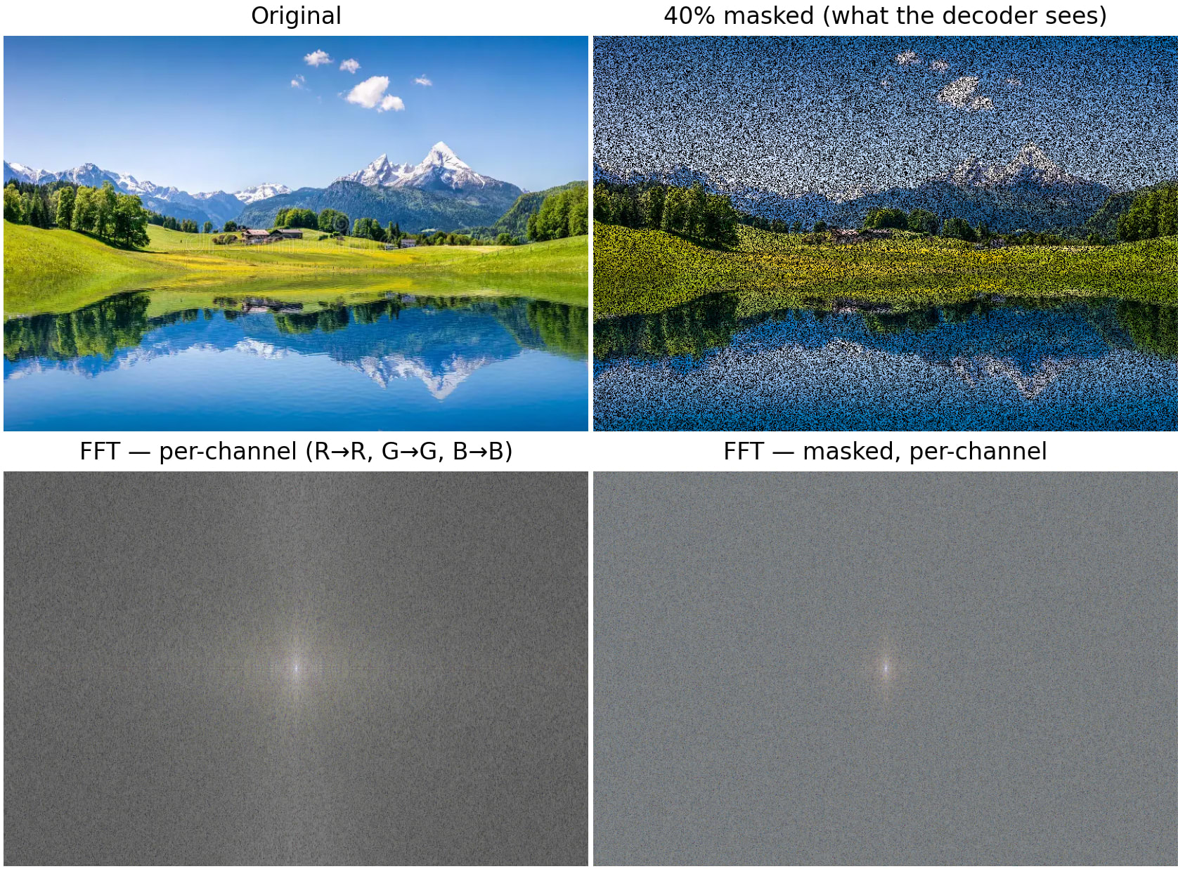
I chose to go for contrastive training, with positives defined as different chunks from the same document. It’s basically free, as long as you ensure that there are enough positives in each batch, which is quite an interesting batching problem22. This contrastive term draws chunks closer if they are from the same document, and pulls them apart if they come from different docs. The effect is that the encoder needs to encode something like “this chunk looks like something you would find in that type of documents”, which is an inherently low-frequency type of information. In the image analogy, it would be like ensuring that patches from the same image get encoded quite similarly. The only way to do that is for the encoder to put things like “This looks like a tree. Must be a part of a landscape” into its latent representation, so that the patch gets close to a patch that says “This looks like a sky. Must also be part of a landscape”.
I have not tested the real-world contribution of this contrastive loss term, though. I just noticed it did improve the effective dimensionality of the CLS space.
</deep_dive>
Here are results of the training23:
Giving a deceptive CLS token barely moves the decoder’s text accuracy. The vast improvement over the encoder-only baseline come from the facts that:
The MLM pre-training of the encoder was done at a fixed 15% masking rate. So it has no idea how to handle 80% masked inputs
The CLS carries basically all the numerical information, leaving more “mental space” to the decoder for text prediction/memorization
On the other hand, the CLS carries nearly all numerical information. At 15% masking rate, the numeric reconstruction is perfect (the loss floor is 0.5, see footnotes). At 85% masking rate, it’s nearly the same as the encoder’s at 15% masking rate.
The conclusion from this auto-encoder training is that the text content of SEC filings is very light on information. And that most of it is still mostly understandable at 80% masking rate24. Most of the information density seems to be in the numbers, and that’s why the encoder focuses on them25.
Checking how the embedding model performs
Nice reconstruction results don’t necessarily mean good real-world results. So, I decided to test the model on 2 custom benchmarks:
A kind of STS benchmark: 20 pairs of paraphrased financial sentences. Testing recall@1 and MRR. The code speaks for itself.
A kind of numerical ordering benchmark. Code speaks for itself. The idea is to check if the model is able to understand that “Last year revenue was $17 billion” is closer to “Last year revenue was $15 billion” than “Last year revenue was $1 billion”. 29 examples.
The model performs surprisingly well despite its lack of task-specific fine-tuning.
It lags BGE-base-v1.5 on pure semantic similarity tasks, but it blasts it (and every other embedding model I’ve tried) on numeric tasks.
We could vastly improve the performance on these specific tasks by fine-tuning the last layer of the model for them26.
Step 4. Embedding whole documents
Step 3 was the tricky one. Step 4 is the “how the heck can I train this with such a small dataset and less than $1,000 of compute?” one.
ModernBERT, that my financial models are based upon, only supports a context length up to 8,192 tokens. Some SEC filings are longer than 128,000 tokens. 16x-ing a context window is possible but quite boring, and it necessitates fine-tuning. Nothing insurmountable, but yet another rabbit hole (that I preferred not) to explore27.
So, I decided to go for another, less compute intensive method: aggregating CLS tokens, via another transformer, to be trained from scratch. The idea is very simple: take the CLS tokens from every chunk from one document, feed them into a transformer, and have it output (either via mean-pooling or attention pooling (CLS)) a single embedding.
Things get a bit fuzzy here, because there is no easy way to check whether the aggregated CLS is good. You can’t paraphrase 128K token documents as easily as you can 128 token chunks. You can’t easily decide that such documents are more alike than such others. So, the only things you’re left with are:
Completely unsupervised setups, like JEPA. That we saw doesn’t work too well unless you have a lot of data, with a certain shape.
The auto-encoder setup. That we saw was subject to the dimensionality collapse phenomenon (footnote 13). The participation ratio of the Step 3 CLS is already rather small, at 128 or so. Going for another aggregation step would likely decrease it further.
Completely supervised setup. Training the aggregator (along with a small regression head) to predict the 5y growth rate. Thing is, a small transformer with a 768 hidden dim has at least a few million params. There’s no way you can train it on a few thousands datapoints. Overfitting is a major concern here.
I’ve tried all 3 methods, and tested them all on the end-to-end task, that is, predicting 5y growth.
I was lucky enough that in-distribution prediction (training on 7000 companies, on the 2018-2015 period; testing on 700 unseen companies but on the same period) is a much easier task than out-of-distribution prediction (training on all 7700 companies on the 2018-2021 period, predicting 2021-2025 growth rates). It gave me a sense of how good the CLS representations were.
In all cases, I used a 6 or 12 layers transformer, with the exact same characteristics as ModernBERT, except for the local attention layers (all layers were global attention). Around 50M params.
The completely supervised setup28 instantly overfit. I was expecting that, but you always have a glimmer of hope. Nope.
JEPA gave me the nicest output distribution entropy/effective dimensionality29. But the output distribution was really noisy, and it just wasn’t good for in-distribution predictions. The CLS representation was so bad that I had to train the aggregator with a very small Learning Rate (1e-6) and a regularization term (MSE with base aggregator’s CLS) to get acceptable results. I got a .15 correlation between predicted in-distribution growth rates and the real growth rates.
The AutoEncoder setup worked the best. The setup is very similar to that of step 3:
The encoder is the CLS aggregator transformer, that we’re trying to train. Its inputs are CLS representations (as computed by the Step 3. encoder) of all the chunks of each document. The Step 3. encoder is, of course, frozen, and the CLSs are pre-computed. I chunked documents differently for each epoch, and pre-computed all the CLSs beforehand.
The decoder is initialized from the Step 3. decoder. It’s trainable. Its job is to de-noise a single chunk of the encoded document. So, it’s given an aggregated CLS representation of the whole document, but its job is to only de-noise a chunk of it.
Once the CLS aggregator has been trained30, it is frozen and a (trainable) regression head is added on top, to predict growth rates. The dimensionality collapse actually was a blessing here. When you have few datapoints, it certainly helps to fight overfitting. I got a .20 in-distribution prediction vs. actual correlation with this setup.
Unfortunately, the .2 in-distribution correlation didn’t translate to any out-of-distribution predictive power. Literally 0. You can check the much more detailed results here31.
Is out-of-distribution prediction even possible?
When I realized that 2018-2021 and 2021-2025 actual growth rates were completely uncorrelated (0.0047) I thought that it would be difficult to predict. Unfortunately, I realized that after I had finished training the Step 4 model.
These growth scores being uncorrelated is perhaps the strongest indication that the task was simply impossible. It doesn’t simply mean that there is probably no signal to be found in the filings, but also that most explanatory variables are extrinsic to the company. If there’s something that makes companies grow for 3 years (say, a certain leadership style, the quality of its marketing department, an engineering moat), it’s statistically unlikely to make it grow for 3 more years. Maybe it’s about the 2018-2025 period specifically, but it shows how nearly impossible this task was.
On the other hand, I was able, with a lot more (structured) data, to actually predict some things that are quite similar to growth rates, and reported the results in a previous blog post.
So, I believe the conclusion is:
2021-2025 growth rates are inherently impossible to predict with a model trained on the 2018-2021 period
But it might still be possible to predict them on different periods, with a lot more data and compute.
Step 3 and Step 4 models work incredible for quantitative data extraction
You can actually use step 3 and step 4 models and training pipelines for a wide variety of quant tasks. It just happened that OOD company growth rates are impossible to predict from SEC filings.
So, I wanted to check how good the model was at extracting table data and reconstructing a clean, structured vector from the CLS representation.
The only part of the filings that is identically structured across filings is the web stats section, that consists of 2 tables, that you can check the structure of here.
So, I PCA-ed the website stats across all filings down to 90% variance explained, which left me with 28 components.
Then, I encoded the Website Statistics section with the Step 3 encoder, and built a small MLP to try to reconstruct the 28-dim structured vector from the 768-dim unstructured CLS embedding. Code is here (and here for the vanilla ModernBERT baseline).
Here are the results:
So, the 150M params encoder, that was never fine-tuned for this task (and was fine-tuned for a total of 10 5090-hours (or 6 H100-hours), is able to encode 54% (0.6 (R^2) * 0.9 (PCA variance explained)) of the quantitative information of a filing section. That’s really cool.
By the way, I am surprised that ModernBERT does a decent job too, despite its dubious number representation: it still encodes 42% of the information. I believe this good performance comes from the high proportion of small integer numbers in this section, that ModernBERT can tokenize and represent soundly. It is likely to be much lower for actual financial tables.
Conclusion & a few technical takeaways
Step 3 and Step 4 models are very good for quantitative feature extraction from unstructured data. Unfortunately, my end goal of predicting company growth rates from their filings wasn’t attainable.
I’ve learnt a bunch of things along the way:
If you need a transformer to understand numbers, use a custom number embedder/prediction head. It just won’t work otherwise (I tested numerous embedding models up to 8B, and they all sucked).
Clean up your data. It’s more important than everything else.
JEPA and other ‘completely unsupervised’ methods don’t work too well with text, because of how small the long-range dependency between text tokens seems to be (compared to image patches). Consequence is that, if you need to embed very long documents with a uniform information density, mean-pooling chunks embeddings might be okay32 (my aggregator transformer might not have been that necessary after all).
Beware the frequency bias of text auto-encoders.
Beware the dimensionality collapse effect of transformers.
Test the feasibility of an idea before throwing 1,000 hours and a few hundred dollars of compute to it. Or don’t, if you want to have fun.
Use git diff and zlib compressed : uncompressed ratio to increase and assess website pages information density. (Seen Annex - Websites)
Total compute used was around $400. Reproducing my results would cost less than $25. 16:1 ratio…
By the way, point 3 and 4 make me think that the LeJEPA way of creating views by cropping images probably puts a lot of emphasis on the lower frequency informations (where most of the information lives anyway, so it’s not too bad for standard image classification tasks). It could be problematic for image tasks where texture and other high-frequency information matter. If I have time, I will investigate a views creation algorithm which frequency bias aligns with the end classification goal. I was thinking that image masking via an Ising model (with a careful, task-specific temperature setting) could be nice. I’ve not given it too much thought though.
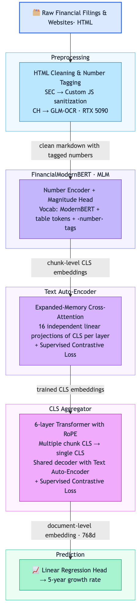
What the project looks like, in the end:
Annex: How I got the data and sanitized it
Claude Code helped a lot. I decided to only use free Anglophone companies data. Namely: SEC filings and Companies House filings. They were all available for download quite easily. I got them for 3 separate years: 2018, 2021 and 2025.
Then, I used CommonCrawl and the Wayback Machine to scrap the 20 top pages from each company website, after matching the company filing and websites using either SEC data, or gemini-flash-lite for the companies house filings (less than $5 for 5,000 companies). I intended to use the full website text as input data, but decided to use only stats (like the ratio of text length to html code length, as a proxy for how bloated the page is) for a first proof of concept.
A few tricks that I used to sanitize the HTMLs (SEC and Companies House Filings, and websites were all HTML):
Websites:
Git diff on all website pages vs. the landing page. Helped remove redundant headers and footers.
Removed all boilerplate pages with a regex on the url. (like ‘legal’, ‘privacy’, ‘cookie’, ‘sitemap’, ‘login’, ‘wp-admin’…)
Filtered out pages with low information density, using the gzip33 compressed size : uncompressed size ratio as a proxy for information density. Problem is: the longer a text, the more compressible it is. So, I built a baseline curve from Wikipedia articles: for each text length (100B to 1MB), what’s the “normal” compression ratio for natural language? Then for each page I compared its compression ratio to the baseline at that length. I was quite happy when I saw that the compression ratio very nicely aligned with my intuition of how dense a page was34.
SEC filings:
Sanitized tables using custom JS injection into a chromium headless browser. When you inspect a SEC filing table, the HTML is horrendous, but it can actually be sanitized programmatically if you take colspan and rowspan attributes into account.
HTML to text (element.textContent) for every non-table section. Easy, that’s it.
Companies House filings:
The HTML of these filings is fucked beyond repair. Nearly all html elements are absolute-positioned. I had to HTML → PDF → OCR → Markdown them. Best OCR model out there is GLM-OCR. I rented a RTX 5090 and used vLLM. It could be a good idea to build your custom SDK, because GLM’s default doesn’t use the GPU fully. My suggestion is: Layout-detect your whole heap of docs, store the bounding box somewhere, then get rid of the layout detection model, then use the “real” GLM OCR model on the bounding boxes, with aggressive vLLM memory settings. You’ll triple speed and GPU usage. I tried it, kind of worked, but I was so frustrated when I encountered a vLLM shutdown midway that I decided to revert to the default SDK and just wait 10h for the OCR to finish.
Most of the companies don’t report their income statements. So, I had to infer their growth rates from all the data they reported. The idea was: checking how all their reported figures grew, and weight-average (based on the significance of the said number) them to get a single number. Eg. Employee count grew 15% and asset base grew 12% → growth rate is probably around 14% (weighing employee count a bit more). Script is here and weights used are here.
After that, all numbers were put between <number> and </number> tags (that the model’s tokenizer understands).
ModernBERT is the backbone model I used. Multiple reasons for that:
Decent context window (thanks to Flash Attention (although SDPA is now trivial to implement in PyTorch) and Local Attention layers)
RoPE
Small (155M params).
Completely overtrained (trillions of training tokens vs. <1B params)
And I incidentally tested nearly all of them in my different experimentations.
Fuck, for some reason, it got changed by Claude Code to -12, 12. I should have checked the default config. The model works okay anyway, but it’s definitely sub-optimal. A few lost flops. From my experience, though, changing the number of bins from 64 to 128 only yielded marginal improvements, so I believe this wasted (-12, -3) range doesn’t have too much impact.
weight_upper = norm_pos - lower_idx.float()
weight_lower = 1.0 - weight_upper
emb_lower = self.magnitude_emb(lower_idx)
emb_upper = self.magnitude_emb(upper_idx)
interpolated = emb_lower * weight_lower.unsqueeze(-1) + emb_upper * weight_upper.unsqueeze(-1)
I think it wasn’t the best call, because it allows a fair bit of non-linearity AFTER the last hidden state. This increased post-hidden-state expressivity decreases the relevance of simple operations on these vectors (like mean pooling or cosine sim computation). Just like averaging 2 numbers before they get exponentiated will not give you a good idea of the exponentials average. I just didn’t want to re-train my model after I figured it out. Plus, the expressivity of the prediction head is still much lower than that of the 22 transformer layers before.
15% mask prob. When masked: 80/10/10 strategy: 80% of the masked tokens get replaced by [MASK] (or a special magnitude bin that I reserved for this purpose, in case of numbers), 10% get assigned a random token (or number), 10% are unchanged.
But if you’re interested nonetheless, here they are: ModernBERT’s loss (only text tokens were masked) on text is 0.65; My model’s text loss is 0.5 and its number loss is .85. Please note that the number loss floor is around .5, considering that the irreducible entropy of the soft-label targets (due to the bin interpolation) is around .5 nats (for a uniform distribution). But, due to {2016, 2017} being a fair chunk of the numbers to predict (and falling quite exactly inside one of the 128 bins), the actual entropy is a bit lower.
2 highlights, though:
I tried using 2D RoPE for tabular data (that make up a good part of financial data), because I didn’t see how 1D RoPE could handle it. I was really proud of the engineering behind my 2D RoPE implementation. But it turns out that 1D RoPE works fine, as long as cells and rows are clearly delimited. I suspect that tokens in a cell somehow get to carry the information of “how many tabs there are between them and the last line-break”.
You absolutely need to minimize padding wastes during training. Claude Code is biased towards bucketing the sequence lengths. That’s bullshit. Just order all your sequences by length, and greedily construct batches before shuffling them. SDPA makes memory usage ~ O(total_number_of_tokens_in_a_batch), so the greedy algorithm is straightforward.
In fact, an encoder transformer can serve as a sequence embedding model right after MLM pre-training (via mean-pooling or attention pooling (CLS, in case of BERT) of the last hidden states), and is usually decent at it. But it can be improved via specific fine-tuning techniques.
The [CLS] token is prepended to every sequence in BERT models. It’s supposed to be the representation of the sequence. It is not trained during MLM, so its hidden state defaults to being quite close to the mean pooling of the other tokens’. But when you train it on sequence-level tasks, it becomes much more interesting.
The mathematical concept is really simple:
Compute all pairwise cosine similarity (both positive and negative pairs) in your batch, so you get a 2D matrix
Softmax each line to make them a probability distribution
Just take the log likelihood of the positive pairs and turn it into a loss.
Result is: pull negatives apart, draw positives closer together. As a consequence, it also results in a higher effective embeddings dimensionality (measured by their participation ratio).
You could argue that “To be or not to be, that is the question” and “Life sucks, why did my father die?” can be positives, but you shouldn’t expect the resulting embedding model to care much about style.
When you think about it, there’s also a bit of bias baked in the JEPA training objective. It’s “on average, you can crop an image and still preserve the subject” or “no big deal if you mask a few tokens in a sentence”. But this bias seems acceptable to me.
MSE: 0.1, SIGReg: 10. The latter depends on the number of views and random projections, so it’s completely useless as a standalone. SIGReg loss at the beginning of the training was around 150.
Just check how erratic the euclidean distances are between similar pairs: benchmark results. Said similar pairs are here.
15-85% uniform mask_prob sampling.
In favor of bidirectional decoder:
Decoder can be initialized from the encoder. Only need to add cross-attention layers.
Autoregressive decoders tend to rely too much on context (they see all of it), which sucks. The only thing the encoder needs to encode is the beginning of the sequence and what can’t be inferred from context. I don’t think such an inductive bias would yield a nice sequence representation.
In favor of causal decoder:
Autoregressive decoder’s training is more elegant. Contrary to bidirectional transformers where only the ~15% masked tokens yield gradients, 100% of causal decoder tokens give training signal.
And I’ve tried a shit-ton of them. Memory Slots Expansion (Claude’s idea) got me to 1.7 loss (text + number) approximately. Here are what my “better ideas” yielded:
Using simple MLPs and fancier setups to directly update the decoder’s tokens based on the CLS token. So, no softmax attention involved. Best loss: 1.8
Component-wise softmax attention scores and values updates. It was painful to implement, and it worked no better. Best loss: 1.8 too.
A lot more memory slots (256), but much smaller rank individual projections (64). Best loss around 1.75.
Using full-rank Memory Slots transformations, but sharing the weights across layers. Allowed to use more memory slots for cheaper. This one was actually quite good. Parameter-wise, it was better than the brute force solution. But param count was never an issue. Compute was, and despite some possible optimizations (like pre-computing all memory slots for all layers (as they were shared across layers)), the increased attention computations (more memory slots => longer sequence length) far outweighed them. So I didn’t investigate further. Best loss around 1.7 too. But with more flops.
I was revolted that Claude came up with the best solution right away, especially considering how fishy 16 full rank independent per layer projections look at first sight.
20 or so, IIRC? For a 768-rank transformation, that’s just as small as it can get.
Sort chunks by length and document id, and greedily construct batches (it’s quite similar to tiling a 2D space).
~66% text accuracy at 80% masking rate is indeed telling.
When I think about it, the fact that I weighed the number loss and text loss equally during training could make this a bit of a self-fulfilling prophecy. Indeed, numbers only make up 8-9% of tokens in an 10-K filing (a bit more in companies house data), but account for ~50% of the loss, by design. From my experience, though, changing the lambda of different loss terms only barely changes their final magnitude. So, small caveat here, but I believe the conclusion holds.
And actually, a slightly better (in terms of val loss) checkpoint of the autoencoder performed slightly worse on both benchmarks, showing that fine-tuning for the end tasks is indeed necessary.
My first concern would be whether a single RTX 6000 Pro (or an H100) would fit ModernBERT + 128K context. I’m pretty sure it would have been able to during inference (easily), but training memory usage was already quite high at 32768 tokens / batch… Nothing insurmountable either (easiest solution being using multiple GPUs, before optimizing anything).
Also, and mainly, fine-tuning at that length necessitates documents that are also coherent at that length. Which is really difficult to find/build, especially in the financial domain. Plus, the usual lack of long range dependency inside long documents (Code is really an outlier in this domain) would just teach the model to come up with a kind of sliding window attention.
Untrained transformer + regression head.
Input: Step 3 CLS tokens,
Output: mean pooling => growth rate.
Loss: MSE on growth rate.
Participation ratio was probably a bit over 100. Average cosine sim was basically 0.
Something that I am surprised didn’t work: As all the models (Step 2, 3 and 4) had been trained on 2018 data, but were tested on 2021 data, I thought it would be a good idea to adapt 2021 aggregated CLS embeddings to make them more “2018”. So I fit a linear regression on 2021 agg-CLS vs 2018 agg-CLS before feeding them into the regression head. It helped with dialing down the average growth rate prediction (so the model may have learned something after all) to make it closer to the actual 2021-2025 median, but it didn’t help at all improving the prediction vs. actual correlation.
The idea is that, if there are no long-range dependency (and interaction) in “normal” text (code is not “normal” in that sense), the whole is not too different from the sum of its parts. Meaning that, as long as the CLS representation space is well formed, which in itself is very interesting question, averaging the CLSs will give a nice document-level representation.
zlib algorithm, more precisely. Just asked Claude Code what the best text compression algorithm was, and it came up with that name.
If you’re interested, a nice threshold is 0.4 times as dense as wikipedia. Below that density threshold, you get pages that are full of shit. Above, you might miss product lists or things like that, that do contain meaningful information.