Hacking Spectral Bias: Using Carrier Functions to Increase Parameter Efficiency

This title is clickbait, but only to a small portion of the population.

When writing about the Stateful Transformer, I came across some nice ML concepts and discovered a few things worth writing about. This post is quite technical, though I restrained from using mathematical expressions when the concept behind them was explainable with words.

The core idea is that adding a well-chosen function to the target (and subtracting it at test time) can help escape local minima in the loss landscape.

A nice French forest in the Lyon area, where I wrote the beginning of this piece.

Learning curve and learning task

This may seem a bit naive to some of you, but I was wondering if the minimum attainable loss vs. number of layers (with a fixed width) curve had a definite shape, for example if adding a transformer layer would yield a predictable loss improvement.

It turns out it doesn’t. In fact, the shape of the loss vs. number of layers depends entirely on the task to learn, and especially on the spectral decay of the function to approximate.

Let’s check that.

Random points

I tried to fit a GELU MLP¹ to a function defined by random points².

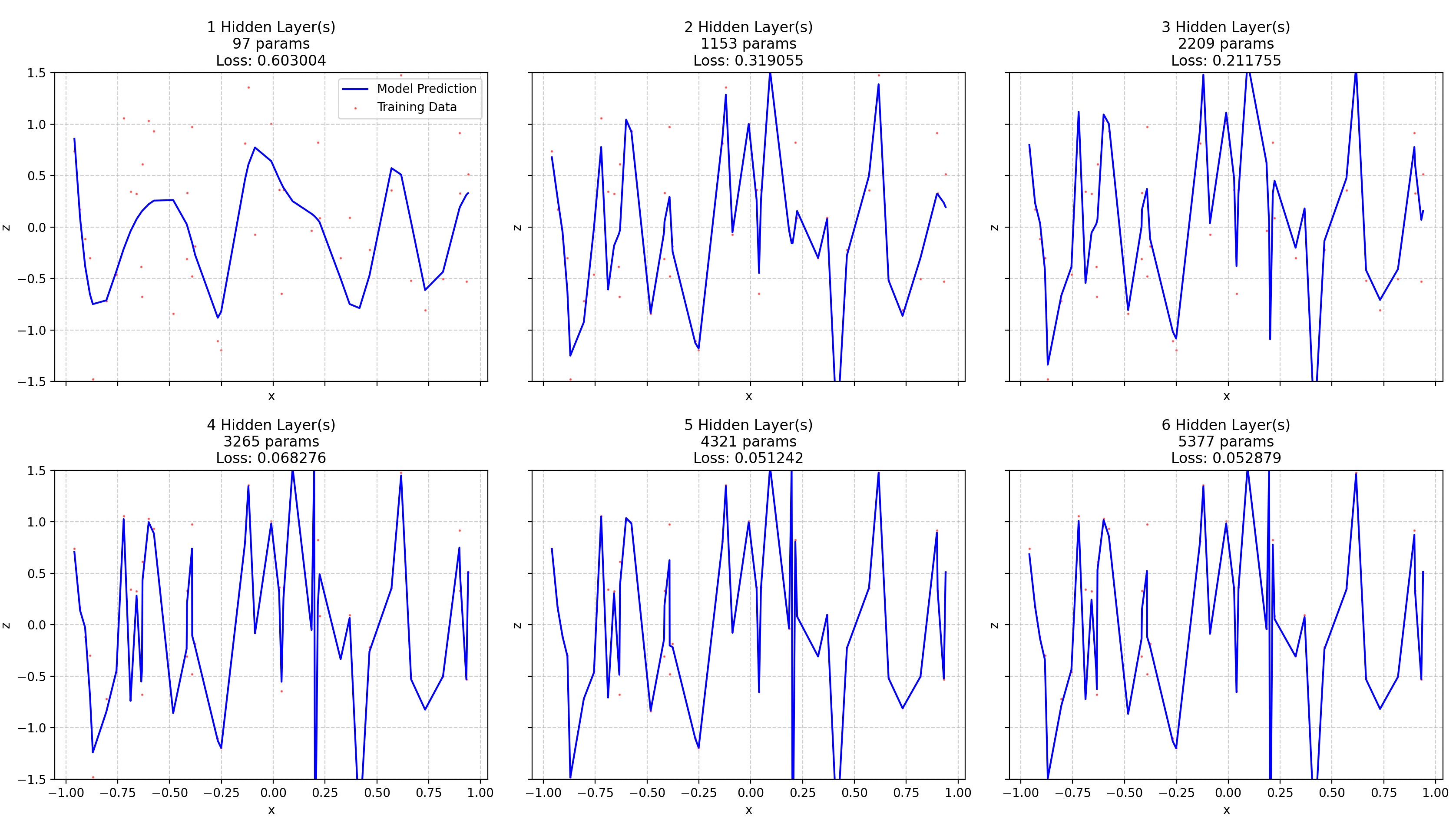
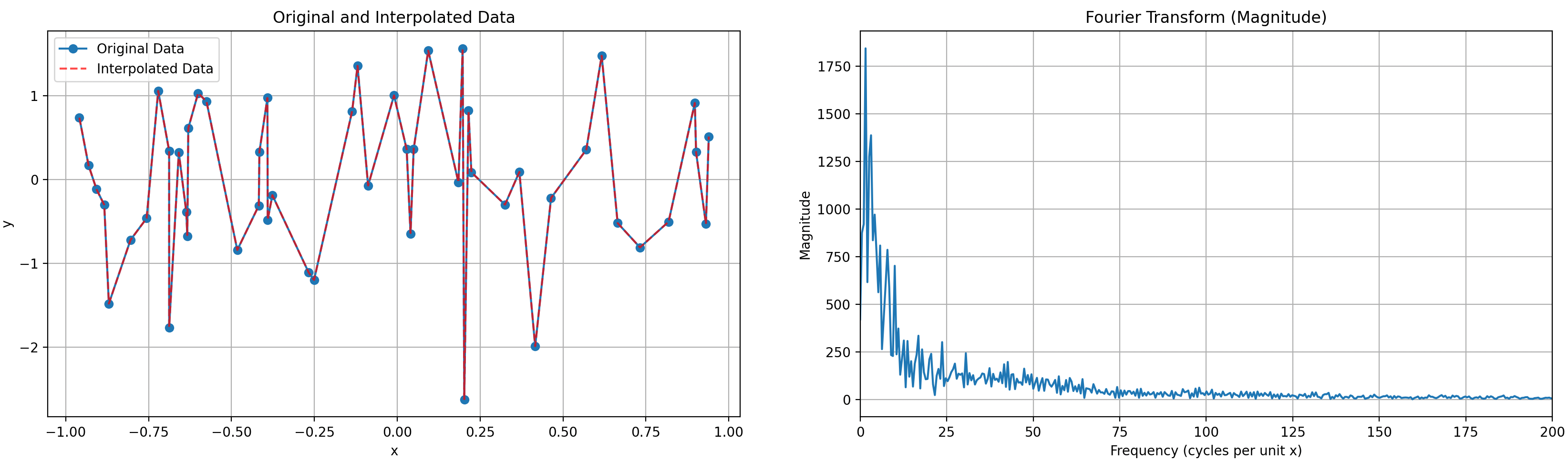
First of all, the random points are not only random on y, but also on x, giving a slowly decaying frequency spectrum (as shown in the next figure) to the function to approximate.

Indeed, if the points were evenly spaced, there would be an obvious frequency peak in the vicinity of {number of points per unit} cycles per unit. But, as the points are unevenly spaced, the frequencies are spread, roughly following a 1/(distribution of distance between two neighboring points drawn from a uniform distribution) law. Which seems quite difficult to compute.

Anyway.

What we can see is that adding layers initially decreases the loss, resulting in early quick wins, until the points to fit are too hard to reach. Then, the loss plateaus. It could go down to 0 if we had a good enough network. But such network seems impossible to get just by increasing the number of layers: we run into training instabilities due to excessive depth before being able to model the hyper-high frequencies of the tail of the spectrum.

Left: the function to approximate. Right: its frequency spectrum.

Variable frequencies

The architecture is the same, but now the function to approximate is cos(15x³). The frequency of this function obviously grows with |x|.

Strong spectral bias observed.

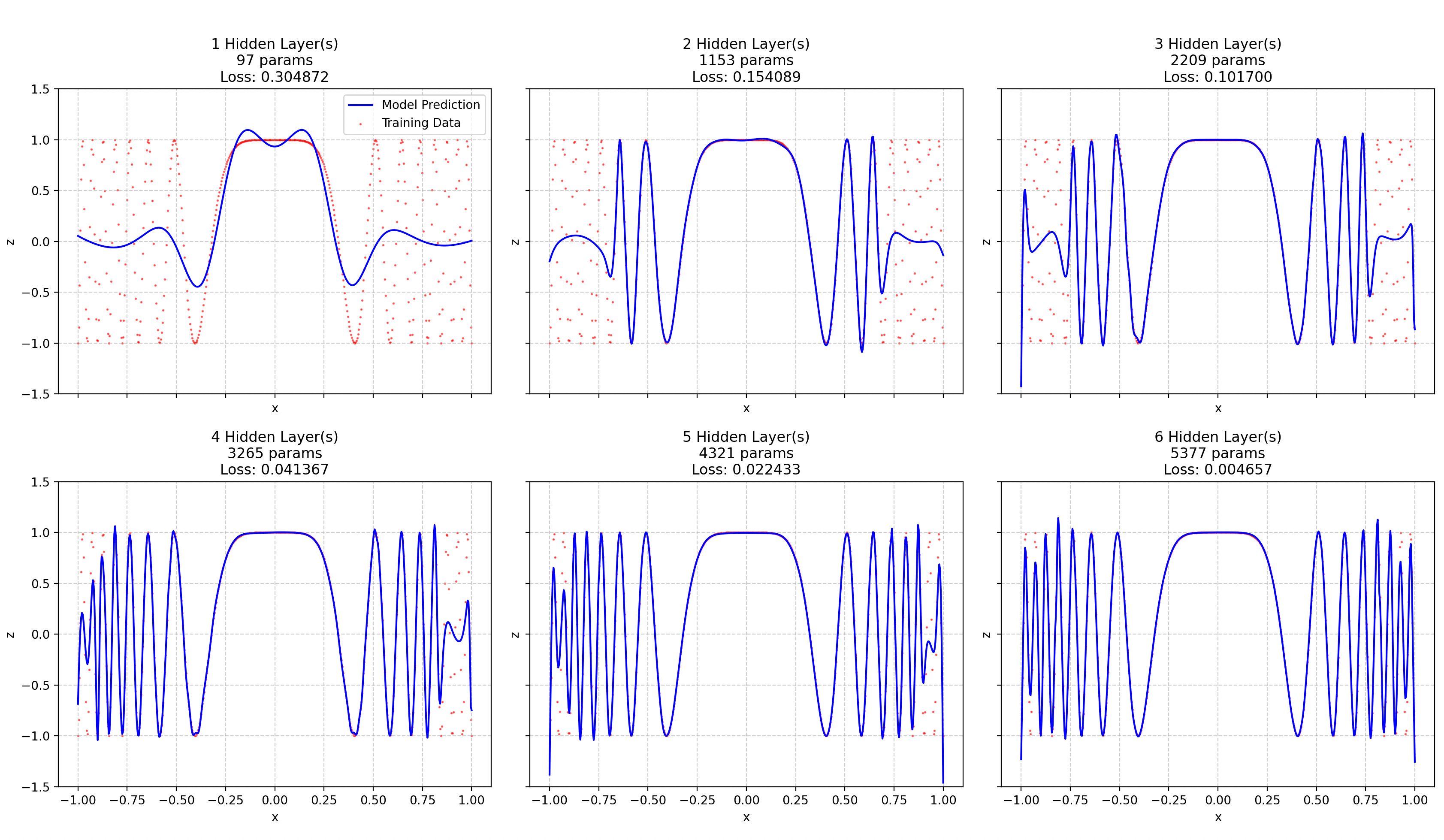
Two things here:

1. The loss is decreasing exponentially (it’s about halved for each added layer until layer 5 and it’s divided by 4 by the last layer).

2. You can see a near-perfect illustration of the spectral bias: NNs have a strong tendency to first fit low frequencies.

Now, the first point basically proves that adding a layer doesn’t have a definite impact on loss, and that it depends on the complexity of the function to model: the loss curve here is dramatically different from that of the random points approximation problem.

The second point is more interesting. Let me digress a bit more about spectral bias first.

The spectral bias of NN has been extensively studied, and the math behind it is sound. But I wonder if real-life spectral bias also has something to do with the fact that, in some cases, the local sample rate of the dataset is not tuned to match the local frequency of the functions to approximate. Let’s take an example.

Let’s say we want to train a CNN to identify animal species based on their pictures. The function to approximate has high frequency regions (felid and bird species sometimes differ only by subtle features) and low-frequency ones (equids are very easy to tell apart: Striped => Zebra. Gray and long ears => Donkey. All the rest => Horse).

If we don’t oversample the high-frequency regions (providing a lot of pictures for each bird and felid species) in the dataset, we are likely to increase the spectral bias of our NN, as a somewhat low-frequency function will do the job of approximating the dataset. Mainly because the total loss on one epoch won’t be frequency-weighted.

This effect is quite obvious so I think it is often taken into account when designing datasets. In financial data modeling, it’s not always the case, though.

Here, the sample rate is constant, and independent of the local frequency. That explains part of the spectral bias.

In the following training runs, the initially evenly spaced datapoints have been spread out by cubic-rooting them, which allows for a sample rate proportional to the signal frequency³.

Despite the fact that the sampling rate is proportional to the signal frequency, we still observe a strong spectral bias.

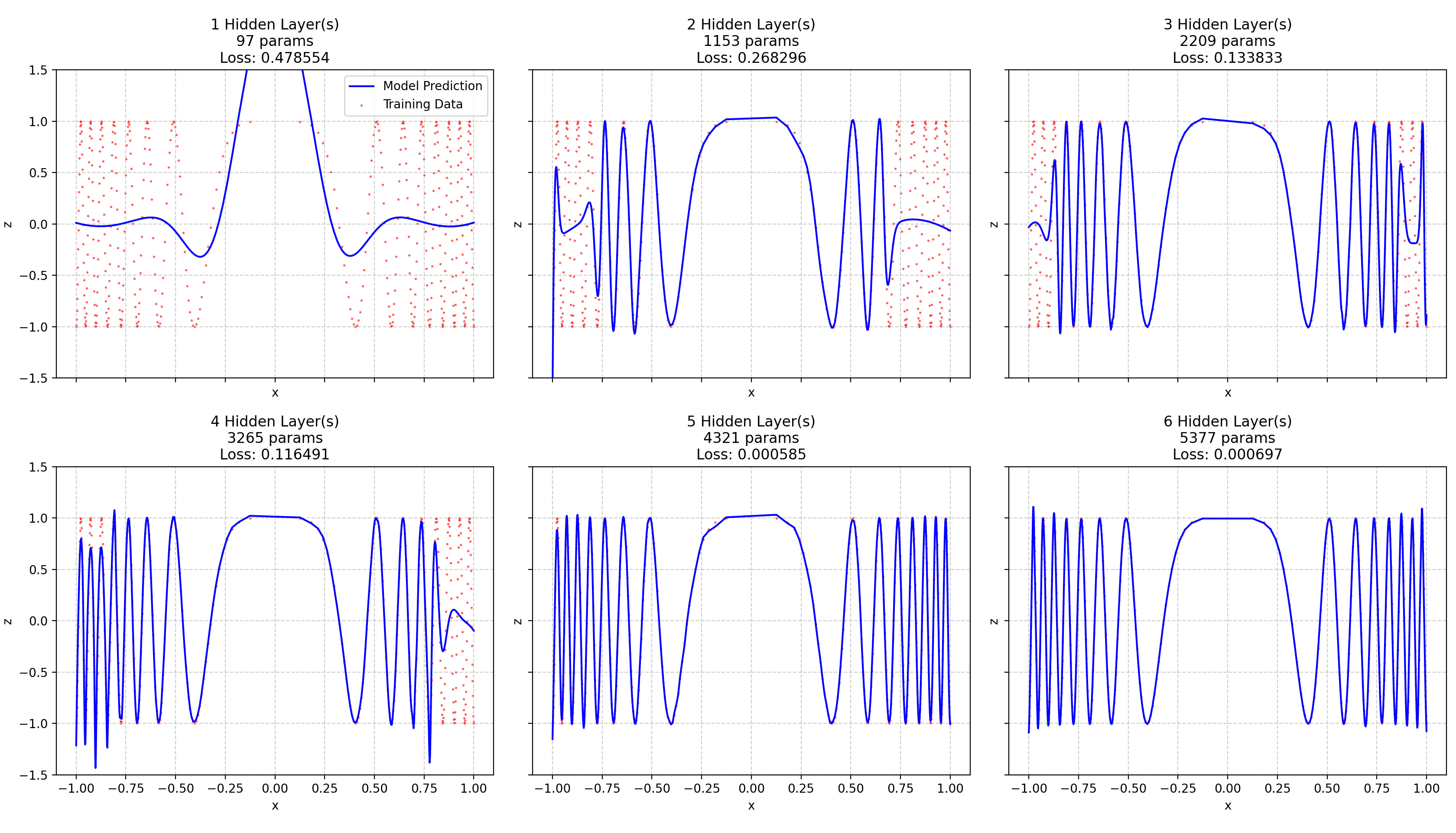
There is still a bit of spectral bias. Also, despite more datapoints being in the “difficult region”, the NN converges quicker.

Enter the edge bias

Next I wanted to see how a GELU network would approximate a single-frequency function (excluding border effects). Would the loss vs. parameter count curve brutally go from one to zero as soon as we reach a certain model size?

I discovered something quite interesting: when you approximate a single frequency function⁴, the extremities of the input distribution are approximated first. Illustration below.

When modeling a pure frequency function, NNs start approximating the function near the extremity of the input domain.

I may be anticipating a bit on the rest, but it all comes down to this: “The frequency of a function composition depends both on the outer function’s frequency and the inner function’s frequency AND amplitude.” It’s pretty obvious if you take f(x) = sin(x) as the outer function and g(x) = a*x as the inner function.

This amplitude/frequency coupling is one of the reasons why the Fourier transform of a composition of functions is intractable.

NNs are a composition of as many functions as they have layers, so this coupling happens a lot.

Let’s try to see why it implies that they are better able to approximate higher frequencies at the border of the input distribution.

The following is not a super rigorous mathematical proof, but I think it gives a good enough intuition of the phenomenon.

Let’s take an underparametrized MLP, trying to approximate the above constant-frequency function.

As it is underparametrized, each layer will underfit its “ideal” transfer function, that is, the transfer function that would allow the whole MLP to approximate the cosine function.

The maximum representable frequency of a NN is basically proportional to the number of “kicks” in the curve (assuming ReLU-like activations), which itself grows exponentially with the number of layers, and polynomially with their widths.

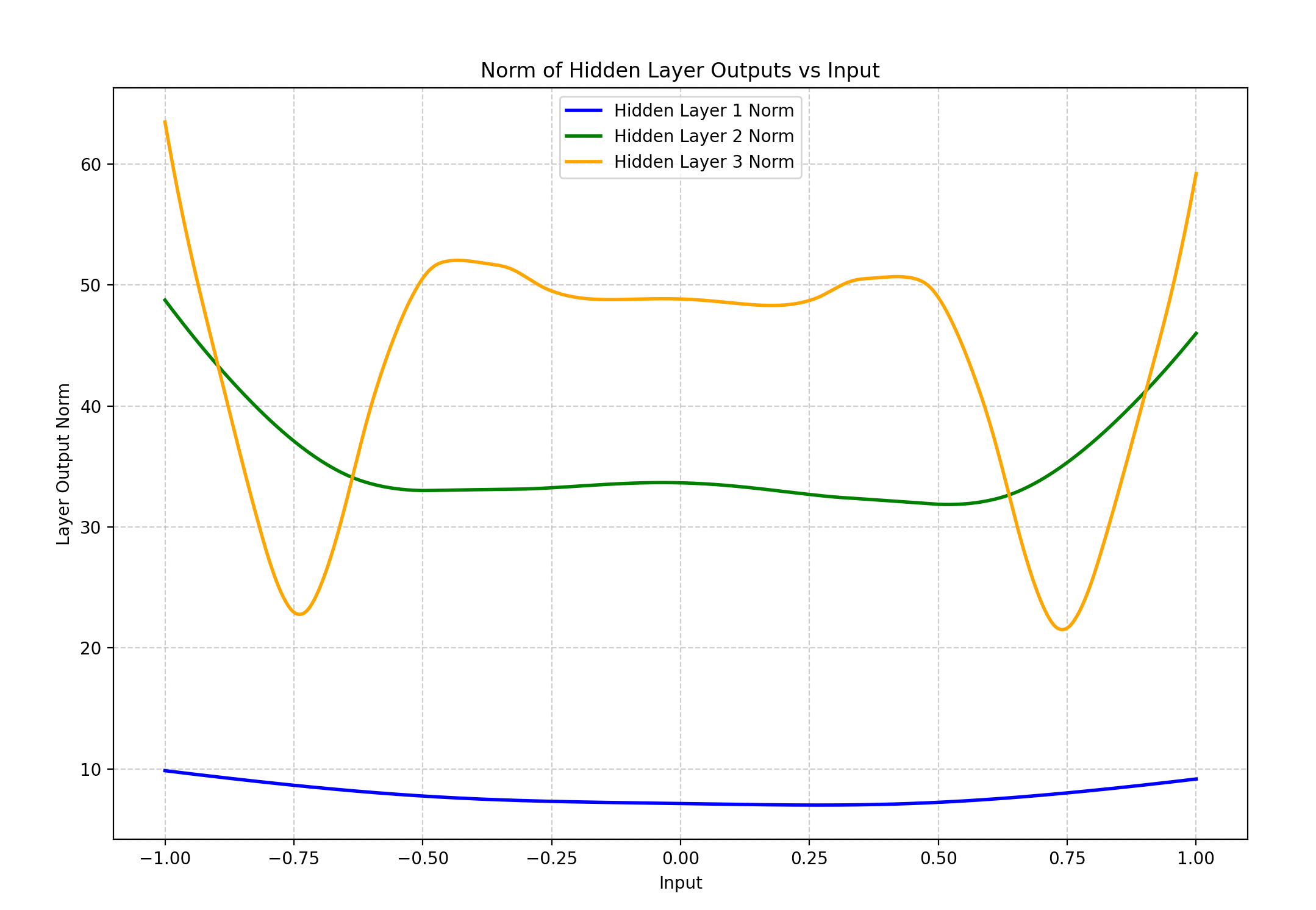
So, for a given trained NN, the maximum representable frequency grows with depth, meaning that if for example we model the frequency of the norm of each hidden state, it likely grows with the depth of our NN.

This implies that the lower layers of the NN, taken together, have a lower frequency function to approximate than the whole NN.

The problem is, as we’re dealing with an underparametrized network, the lower layers have trouble fitting even this low-frequency function. As they are subject to the “normal” spectral bias, they will first try to approximate its lower frequencies.

Assuming our batch size is equal to our number of input points, the backward pass will basically say, for each point: “What is the best nth-order function that models what’s on our left and what’s on our right”. With n a number determined by the width and number of layers at that point. Near the extremities of the input domain, the optimization is less constrained: there is one direction⁵ in which you just have a few points to approximate, and you don’t care what’s beyond these points.

So the lower layers have an easier time approximating their target function near the extremities. Unless the target function happens to be very much biased toward having a lower norm at the extremities of the input domain, that leaves the approximated function with a somewhat higher derivative/amplitude near the extremities.

You may say that the optimization process does not happen layer by layer and that there are no intermediate target sub-functions to approximate, and you’d be right, but my point still holds: the lower layers still tend to yield functions with a higher amplitude at the frontier of the input domain⁶.

Now, given that, in a composition of two functions, a high inner function (ie lower layer) amplitude leads to a higher frequency of the composition, we can infer that the upper layers will have an easier time modeling higher frequencies where their input (ie the output of the lower layers) has a large amplitude. Then, the learning continues inwards to the center of the distribution, but slowly: it’s difficult for the next layer to model a complex function where the amplitude is small. The representable input domain thus slowly grows inwards⁷.

The next layers then inherit a high-frequency and high-amplitude input at the edge of the input distribution and a slightly greater useful input domain. They increase this edge bias even further.

It indeed seems that the edge spectral bias grows with NN depth.

If you have as much trouble understanding it as I’ve had, let me sum up this explanation:

1. The optimization process generally has more degrees of freedom at the extremity of the training input domain, and so for every layer.

2. It results in higher amplitude at the edges.

3. Which translates to higher representable frequencies at the edges, because of the aforementioned Fourier of a composition of functions.

The edge stuff is just the primer of the phenomenon, but the real driver is the amplitude/frequency coupling.

If, for example, I force a low-frequency, high-amplitude, center-heavy component into our function, we find that the center gets fit first⁸:

Now, I find this phenomenon (edge bias + ampl/freq coupling) explains some surprising things in ML. Let’s dig into it.

Edge bias and dimensionality

Now, any seasoned ML scientist would rightly think “So, you’re telling me about edges and you’re using a 1D example to illustrate it? That’s borderline dishonest. Everyone knows that things totally change with dimensionality. Have you heard about the shell effect?”.

Indeed, uniformly distributed high-dimensional vectors are almost always near the edges, due to the “shell effect”. So, maybe this edge bias doesn’t matter much in practical ML applications?

Let’s check that.

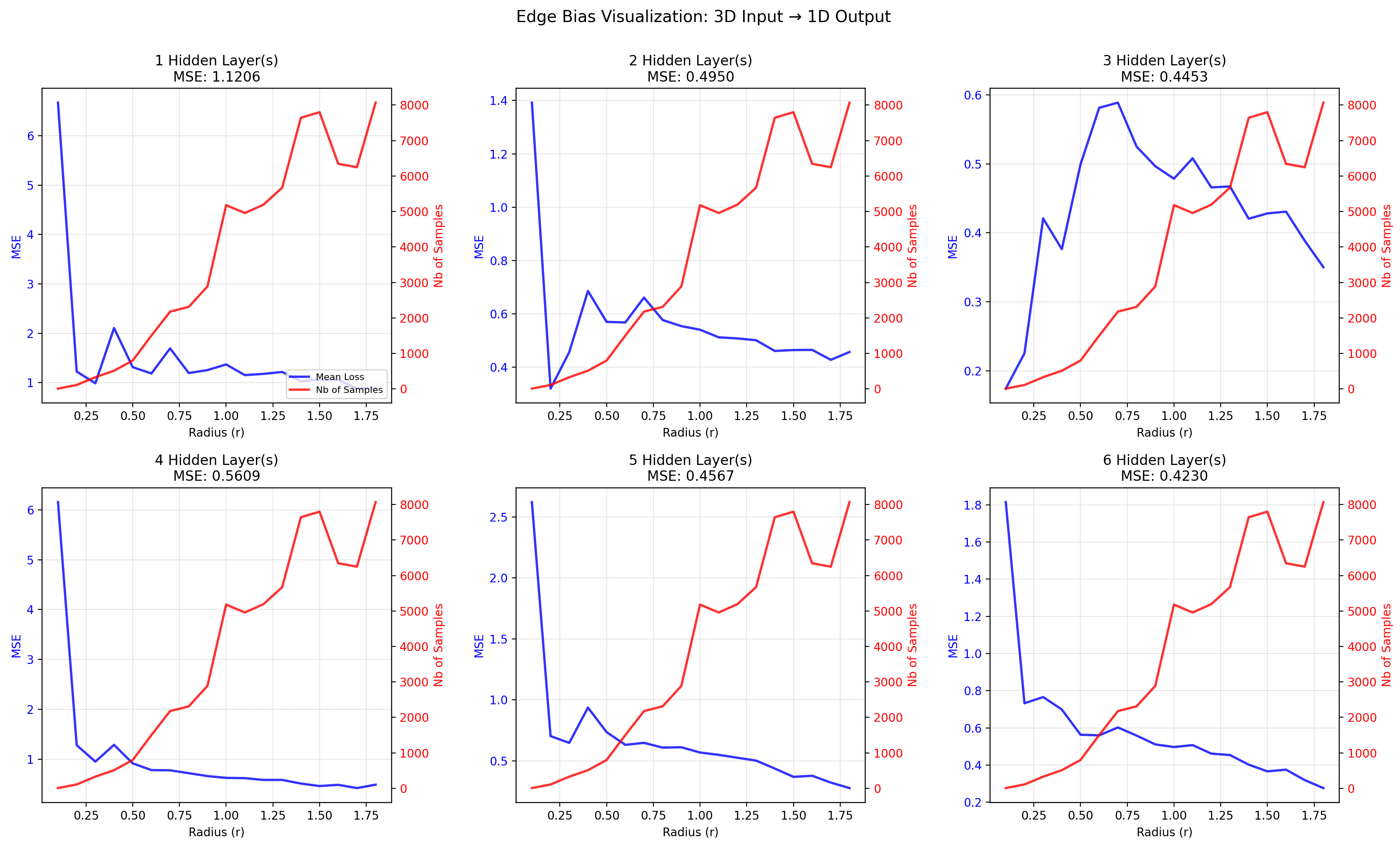
Here is a visualization of 1D and 3D edge biases.

Here, I plotted the Mean Squared Error vs. the distance to the center. Function to approximate is y = cos(x**1.5 * 15). We can see that, with 2 hidden layers, the extremities and the center get fit first. As the edge bias grows with depth, the 3-layer network fits the extremities first and doesn’t care about the center. In red, you can see the number of samples for each 0.1 norm interval. It is not constant because I wanted to make sure the sample rate was proportional to the frequency. The most important thing here is that failing to fit the center leaves a lot of points behind and greatly hurts the MSE on the whole dataset.

Here, the function to approximate is y = cos(x[0] * 7) + cos(x[1] * 7) + cos(x[2] * 7). Still some kind of edge bias: the edges are better approximated than the center. This effect grows with NN depth. Still, it doesn’t matter much, as the center accounts for a negligible portion of the training samples and of the total loss. So there still is an edge bias, but it has less impact.

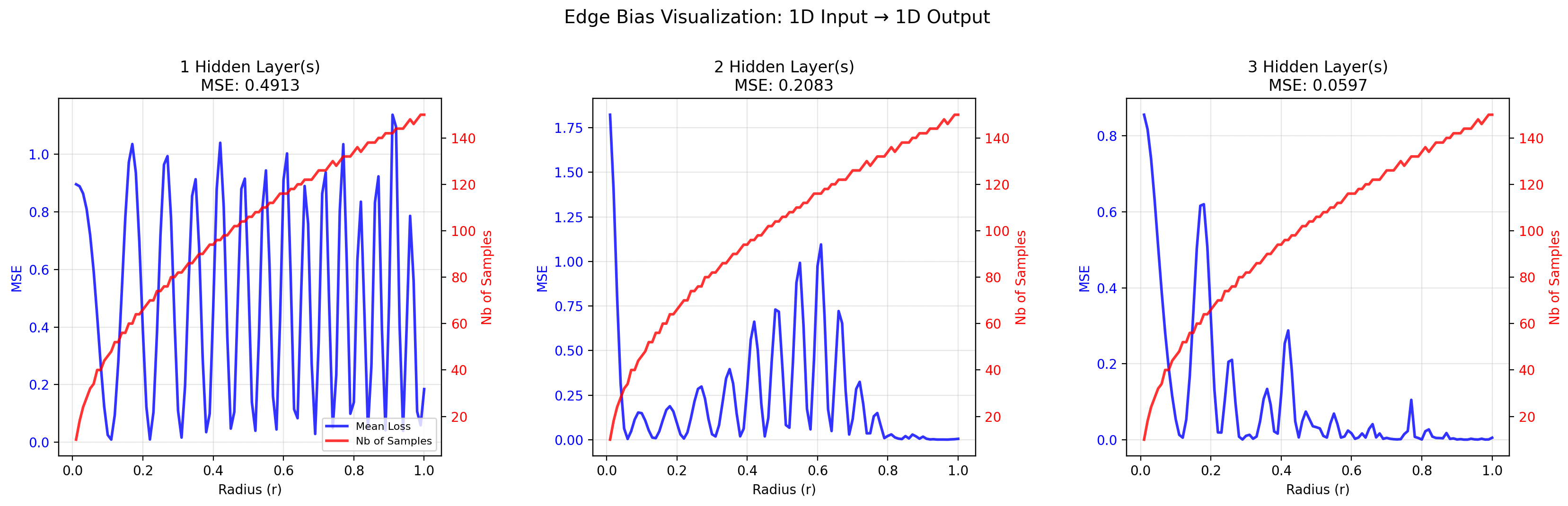
By the way, the definition of “edge” depends on the norm you use. And what’s funny is that the appropriate norm depends on the interaction between the input components. If you expect no interaction at all (ie an additively-separable function), you should use the L1 norm (that’s what I did, as the 3D function to approximate is additively separable). If you expect moderate interaction, you should use an L{moderate order} norm⁹.

Despite the shell effect, the edge bias might in fact be a thing in high dimension:

1. Most real-world functions feature no input interaction or low-order ones. For example, I have heard that genomic studies rarely find interaction between genes. Meaning that if 1000 different genes code for IQ, it is not absurd to model the impact of each gene independently from the others.¹⁰ In financial modeling, which I’m more familiar with, input feature interactions are of a low order, provided you’ve already curated the data and pre-computed useful ratios.
   So, in theory, the norms used to define real-world edges should be low-order ones.

2. Most real world data distributions are center-heavy (eg. normal). So the input vectors comprise a certain number of normally distributed independent input features. And if the features are not independent, then we just have to PCA the input space to make them more so.

3. Using 1. and 2, in the case where we have normally distributed input features and where the L1 norm is the most appropriate (low order interaction), the whole input space shows no shell effect at all.
   Quite the opposite in fact: the majority of the input samples will be very closely distributed around the center, as their norm will be a sum of the absolute value of normally distributed features. I guess it results in a normal(-ish?¹¹) shape for the nb of samples vs. norm curve, surely with a very low sd.
   So, no shell effect at all.
   If we used a very high order norm, L∞ for example, we would get a very strong shell effect, even with normally distributed input features, as the odds of a samples not being at the edge would exponentially decrease when increasing the input dim.

So, the edge bias might still be a thing in high dimension. Please tell me if you have come across something resembling it in your real world ML experience. I have not tested it.

Could be nice to do, but for now, I have a more interesting and practical thing to show.

Amplitude / Frequency coupling consequences: what if we added a function during training and subtracted it for inference?

The idea I want to explore here is that, as high frequencies are easier to model when the amplitude is locally high, what if we add a function whose local amplitude (meaning, its derivative) is high when the target function’s local frequency is high?

Here is an example.

Function to approximate:¹²

\(y = \sum_{i=1}^{3} \cos(7\pi x_i^2)\)

So, the frequency grows linearly with x’s norm.

What if we add this:

\(y = 0.4 \left( \sum_{i=1}^{3} |x_i| \right)^2\)

To get:

\(y = \sum_{i=1}^{3} \cos(7\pi x_i^2) + 0.4 \left( \sum_{i=1}^{3} |x_i| \right)^2\)

Or, if you prefer code, here is our function to approximate:

y = np.cos(np.pi * np.abs(x)**2 * 7) + .4 * np.abs(np.linalg.norm(x, ord=1, axis=1, keepdims=True))**2

The first term is our target function. The second one is useful only in that its derivative is proportional to our target frequency. The .4 factor was just empirically found to be quite good. It’s a bit reminiscent of a “carrier wave” in radio signals.

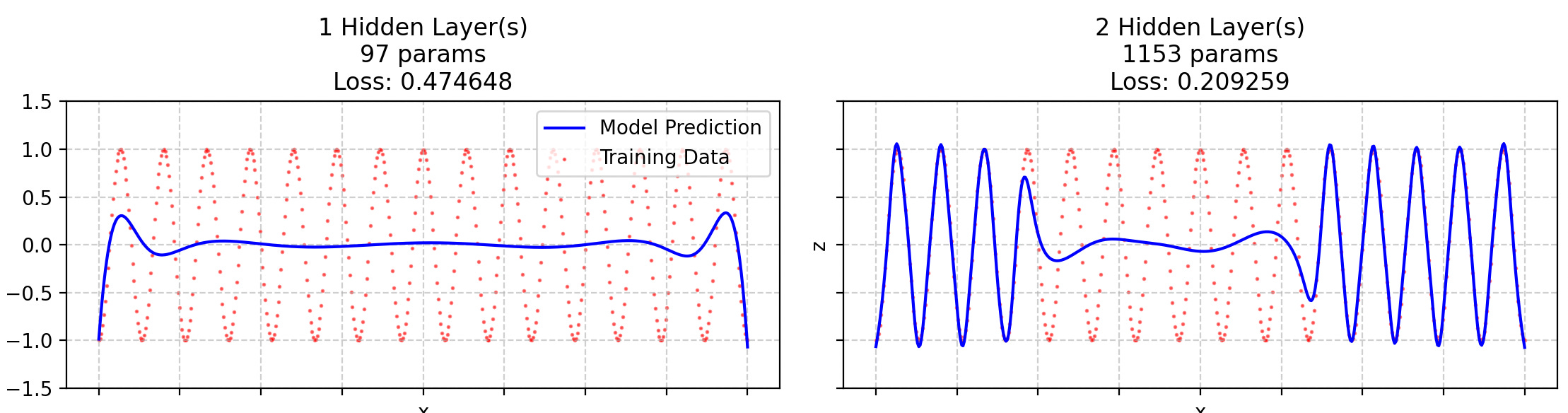
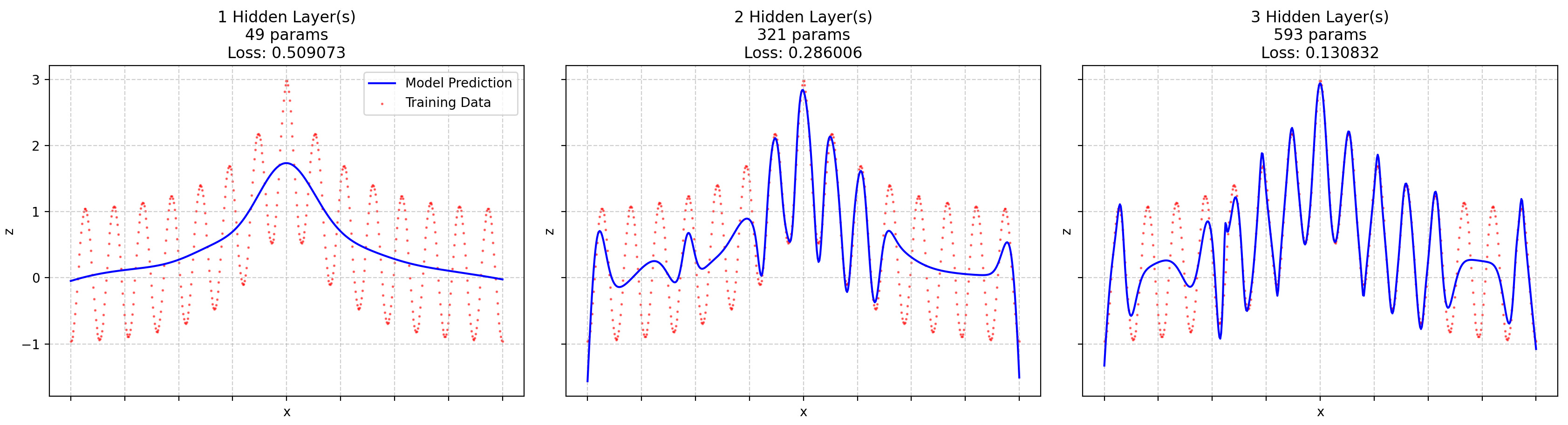
If we train the exact same model¹³ to approximate the target alone or the full function, here are the results:

So, a 1-layer network has a hard time approximating the full function, as it’s a bit more complex than the mere target. Things get easier for the 2-layer NN and the 3-layer one really takes advantage of the improved digestibility of the full function. So, amplitude/frequency coupling really is a thing, at least in this experimental setting.

Interestingly enough, this effect doesn’t hold with even deeper networks. The difference between ‘target alone’ and ‘full function’ losses becomes insignificant past a depth of 4 hidden layers¹⁴.

I don’t exactly know where it comes from, but I suspect 3-layers is the sweet spot between “The additional complexity of the full function makes it harder to model by a seriously underparametrized NN” and “There are enough layers for the lower ones to figure out they should have higher gradients where the expected frequency is high”.

What about carrier function learning?

When we look at the number of parameters of the models and the number of linear regions theoretically attainable by their transfer functions, we can see that they are largely sufficient for approximating our target with negligible error. Backpropagation is just doing a poor job of optimizing them.

The problem comes from the layered structure of Deep Neural Nets.
On the one hand it’s very effective: It enables complex, non-linear functions at a low computational cost. This efficiency comes from two key factors: the chain rule and the way complexity (the number of linear regions) grows exponentially with the number of layers.
So number of linear regions grows exponentially with depth, while training cost only grows linearly. Quite cool.
But on the other hand, it constrains the loss landscape, by making the tuning of each parameter dependent on the others. This results in a loss landscape with an effective dimension far lower than the number of parameters. This, in turn, makes finding local minima much more likely¹⁵.

Adding a carrier function seems to mitigate that, but we are actually cheating here, because we already know where the target function has a high frequency.

So, in real world applications, it would have to be dynamic (if not learnable).

Maybe we could imagine a kind of regularization layer that adds a carrier function to the input of the next layer. This function should not be learnt through backpropagation, but rather through some computation of a proxy for the frequency of the output of the next layer.

But I will write about this later. This blog post is already long enough.

Conclusion / Some key takeaways

1. The shape of the loss vs. nb of layers curve of a fixed-width MLP depends on the spectral decay of the target function. Pretty obvious when you think about it.

2. Real world spectral bias might be partly caused by a failure to match the local sampling rate of the input to the local frequency of the target function. I have no evidence for that though.

3. The observed frequency/amplitude coupling in Deep Neural Nets causes a few interesting phenomenons, including:

   1. A kind of edge bias, where NNs tend to better learn data at the edge of the input domain. This edge bias might keep being a thing even with high-dimensional inputs, depending on the order of the interaction between input components and the distribution of the said input components.

   2. The fact that you can increase the parameter efficiency of a model just by adding a kind of “carrier function” to the targets (and subtracting it at test time).

4. It could be interesting to design a kind of regularization layer based on 3.b.

Researching this was nice. I’ve only scratched the surface and probably have reinvented the wheel a lot, but I’ve had fun doing it.

Notes:

1. Input dim = 1, Output dim = 1, 1 to 6 hidden layers of dim 32 with GELU activation functions, trained for 10,000 epochs on the 50 points with Adam(lr=1e-3, weight_decay=0). Took the loss of the best of 5 runs for each depth.

2. Code for the random points:
N = 50
x = np.random.uniform(-1, 1, (N, 1))
y = np.random.normal(0, 1, (N, 1))

3. N = 500
x = np.linspace(-1, 1, N).reshape(-1, 1)
x = np.cbrt(x)
y = np.cos(np.pi * x**3 * 15)

4. N = 500
x = np.linspace(-1, 1, N).reshape(-1, 1)
y = np.cos(np.pi * x * 15)

5. We are still in the 1D case

6. The graph (and note below) illustrate this categorical assertion.

7. This plot illustrates the phenomenon: the first “kick” in the curve happens closer and closer to zero (the center of the input distribution) as we move deeper into the hidden layers.

8. N = 500
decay_rate = -4
x = np.linspace(-1, 1, N).reshape(-1, 1)
y = np.cos(np.pi * x * 15) + 2.71828**(decay_rate*abs(x))*2
(Yes, I could have used math.exp(1))

9. This is definitely not rigorous. What I’m saying is that the order of the norm used to define the edges should roughly reflect the order of the interaction between input variables. But even if your target function is separable or if the input variables interaction order exactly matches that of the norm you use (eg if you wanted to model the f(x, y, z) = sqrt(x**2 + y**2 + z**2) function), you have no guarantee that the actual transfer function of your trained NN involves interaction of this exact order.

10. In fact, upon closer study, it seems that this lack of observed interaction comes from a lack of data: you need to have a great deal of data points to figure out the interaction between multiple input variables, and there are only so many genomes you can sequence. So, not the best example I could give actually.

11. Not sure of the impact of the absolute value here. Not given it too much thought.

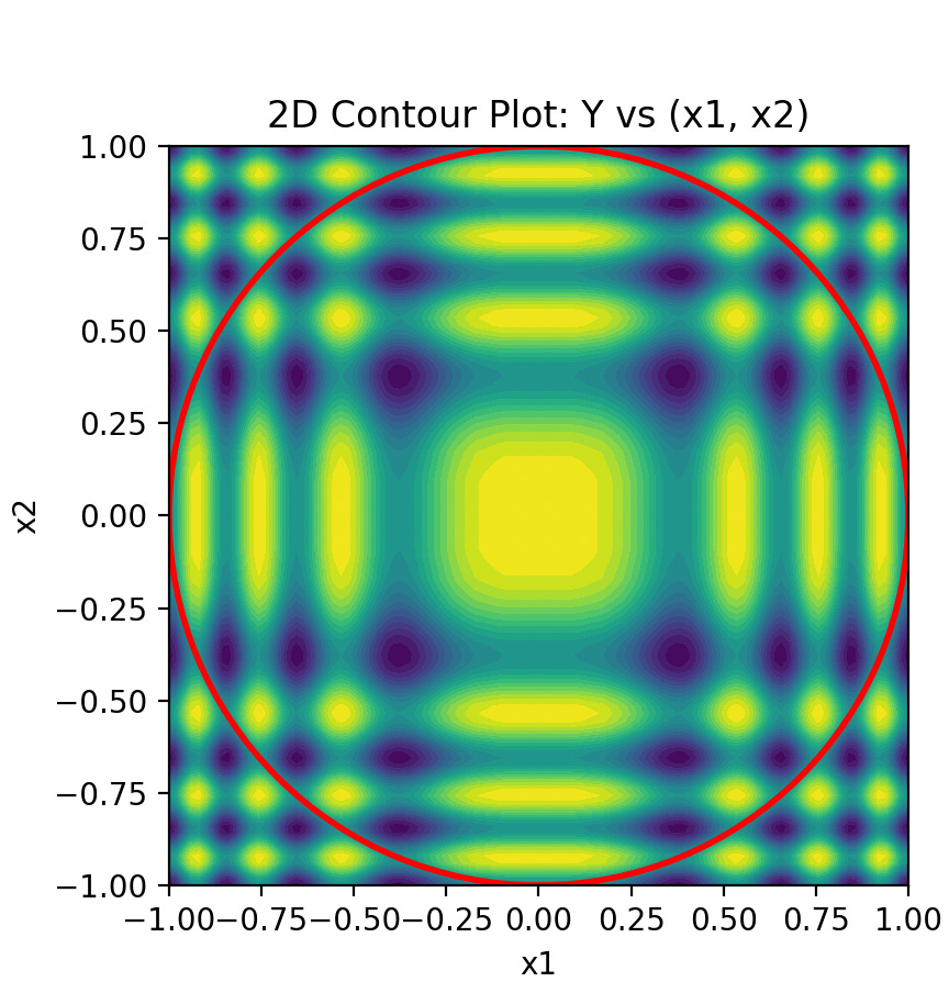
12. Looks like this in 2D:

13. input dim = 3,
hidden dim = 32,
LeakyReLU activation,
1 to 3 hidden layers,
output dim = 1,
1e6 data points, sampling rate proportional to frequency.

14. Oh, and the difference with < 3 layers really is significant, it’s not just a case of “try enough things and at some point you’ll get a significant result”. I’ve done a few training runs with different hidden dims and activations and the same effect can be observed. For example, the results are more impressive with a hidden dim of 64, and seem to remain significant for deeper networks.

15. Indeed, there are far fewer local minima in high-dimensional spaces: the odds of having a positive second derivative and a null derivative of the loss wrt every dimension become exponentially lower as the number of dimension grows. GIVEN ONLY THAT the partial derivatives are linearly independent from one another, which is not the case because of the deep structure of NN.